$130+ Billion in Undisclosed Foreign Exchange Intervention by Taiwan's Central Bank

This is the fifth post in a series* on Taiwan's life insurers and their private & sovereign FX hedging counterparties. It’s the product of a collaboration with S.T.W**, a market participant and friend of the blog. Printable versions of entries in this series are available in pdf format on his site (Concentrated Ambiguity).

Part Five: Searching for Counterparties: The Central Bank of the Republic of China

Taiwan’s life insurers do not fully FX hedge their overseas bond portfolios, but they still have large hedging needs—one that neither Taiwan’s banks nor offshore investors appear to meet completely. The obvious additional counterparty, directly or indirectly, is Taiwan’s central bank (the Central Bank of the Republic of China, or CBC). Taiwan’s central bank, unusually, does not disclose its position in FX derivative markets, and thus its true foreign exchange exposures. But its true exposures can be estimated using similar statistical techniques applied in evaluating an investment fund’s underlying positions from its profit and loss statements. Based on profits and losses which Taiwan’s central bank does disclose, it appears that its true FX exposures exceed its disclosed foreign exchange reserves by USD 130bn, and perhaps as much as USD 200bn. The gap between the central bank’s estimated FX exposures and its disclosed foreign exchange reserves increased significantly after 2011, when Taiwan’s life insurance industry started to rapidly increase its holdings of dollar denominated bonds.

More on:

Taiwan

Currency Reserves

A. The CBC: In its Own Words

Follow the Money

Brad Setser tracks cross-border flows, with a bit of macroeconomics thrown in.

Url

Email

View all newsletters >

Taiwan’s central bank does not supply quantitative information about its activities in the FX swap and FX forward markets, as it—almost uniquely among the world’s large central banks—does not follow the IMF’s reserve template (the IRFCL). But at various times over the past fifteen years, it has hinted at its activities in its annual reports^[1]. Before the global financial crisis, it often noted its activity in FX swap markets.

2003:

• “The Bank carried out swap transactions and foreign currency call-loan transactions to provide banks with sufficient foreign exchange liquidity to meet their corporate clients’ funding needs.”

2004:

More on:

Taiwan

Currency Reserves

• “[...] trading volumes of foreign exchange swaps, options, and forwards all recorded growth rates of above 60 percent. [...] trend that banks tended to use the interbank swap market to adjust their currency composition, and that businesses inclined to utilizing financial derivatives to hedge the increasing risks they faced.”
• “In addition, foreign exchange swaps with banks were used extensively [by the CBC] to absorb excess liquidity.”
• “Moreover, the Bank actively carried out foreign currency swap transactions.”

2005:

• “The trading volumes of cross currency swaps and foreign exchange swaps recorded the highest growth rates of 124.0 percent and 33.3 percent, respectively. The increase was mainly because domestic insurance companies increased their overseas investments and utilized cross currency swaps and foreign exchange swaps to hedge risks, and because banks used the interbank swap market to adjust their currency composition.”
• “[...]some banks used foreign exchange swaps in place of call-loan transactions.”

2006:

• “In addition, foreign exchange swaps with banks were also used continuously to reduce excess liquidity. At the end of the year, its outstanding balance decreased from the previous year, mainly because the needs for hedge by insurance companies declined.”

2007-2018:

• “[...] the Bank continued to carry out foreign currency swap transactions with banks and extended foreign currency call loans to banks so as to facilitate corporate financing smoothly”.
   

Narrative-wise, it is hard to capture the situation better than the CBC did before the crisis. The lifers’ overseas investments increase demand for FX hedges and that demand is accommodated by domestic Taiwanese banks. They in turn use the interbank FX market to adjust their currency exposure. But for the banks in aggregate to reach FX neutrality in the interbank market, a net supplier of FX swaps is required ... and found in the CBC itself, supplying FX swaps to “absorb excess liquidity”. To review, the CBC would typically receive Taiwanese dollars in exchange for USD in an FX swap.

It is unfortunate the CBC has said relatively little since 2006. Back then, demand by lifers was in its infancy. But the central bank’s descriptions of its pre-crisis activity invites questions about the size of its post-crisis exposures.

B. Central Bank + FX Swaps = … Balance Sheet Shrinkage!

A central bank’s FX derivative exposures can, in theory, be estimated based on information it does disclose, even if it does not disclose its full exposures. To see how, it helps to start with the impact of FX forwards and FX swaps on a central bank’s balance sheet. The goal here is to highlight why disclosure of on-balance sheet foreign exchange reserves do not actually show a central bank’s true foreign exchange position if it is active in FX swap markets.

A central bank’s toolbox when it comes to FX derivative markets includes both intervention via FX forwards and FX swaps. Of these, FX forwards provide the most flexibility. They can be entered outright, deliberately creating FX exposures, or in conjunction with an asset to be hedged, then resulting in an FX neutral package. FX swaps formalize this neutralization by conducting the spot and forward transaction with the same counterparty, a process best described as symmetrically collateralized lending. Because of the logistical ease of this pairing, hedgers typically show a preference for FX swaps, while outright FX exposures (including FX interventions) are usually conducted via forwards^[2].

With this is mind, it would seem sensible for the CBC to intervene in FX derivative markets using FX forwards, with local banks as counterparties. If intervention occurred that way, it could be termed a ’pure derivative’ intervention since, upon initiation, a forward transaction entails no exchange of principal. This contrasts with FX swaps or cross currency swaps, which do. Given that forwards are traded in the over-the-counter market and the CBC does not release detailed information about its FX reserves using the IMF’s IRFCL template, such exposures would remain effectively hidden.

However as the previous section has shown, the CBC relies heavily on FX swaps^[3]. Although the use of forwards and swaps is rather different for private sector institutions, it turns out that for central banks, the balance sheet impact of an FX swap is the same as the balance sheet impact of an FX forward. This is due to the accounting treatment of domestic currency on the liability side of the monetary authority’s balance sheet.

Why this is the case is best illustrated by a sequence of stylized T-account examples.

Fig. 1 shows the highly abstracted baseline condition of a four sector model of Taiwan’s economy, including the CBC, the banking sector, households and life insurers. In all examples, the USD/TWD exchange rate is arbitrarily set to 30. In this state, the only prior action which has occurred is an accumulation of USD 100bn FX reserves by the central bank. The reason for this intervention was limiting upward pressure put on TWD by a large current account surplus. It is assumed that the CBC holds these dollars on deposit with a bank outside Taiwan, which is thus not shown in this model. During the intervention, the CBC took USD from foreigners and gave them TWD, which they in turn used to acquire Taiwanese goods. Ultimately, these funds ended up with the household sector, paid out as wages by firms producing the products sold. Households deposit these TWD 3000bn with the banking system (corresponding assets & liabilities marked in the same color, in this case purple). For banks, these represent excess funds, created by the CBC’s FX intervention. As such, the banking system is flush with excess funds on its asset side, which it (has to) redirect(s) to the central bank, which is providing the banking system deposit accounts for excess liquidity^[4]. The insurance industry has not entered the game yet.

Fig. 2 simulates what happens when the CBC again intervenes in FX markets, but households this time acquire a life insurance policy instead of just holding deposits with banks. Importantly, in this intermediate stage, lifers do not yet invest abroad (which comes next), but hold deposits instead. Starting on the left side, the CBC again intervenes in the FX market to counter a large Current Account surplus, which would push TWD upwards. The volume is again USD 100bn, the equivalent of TWD 3,000bn. Households receive this latter sum and purchase life insurance policies (red). Lifers deposit the amount with banks (blue), which in turn increases their deposits with the CBC by TWD 3,000bn to TWD 6,000bn.

Fig. 3 seeks to depict the complicated dynamics set off when lifers start to acquire FX-hedged USD-denominated debt. Starting on the right hand side, a lifer decides to structure its FX neutral overseas investments via FX swaps, which it requests a quote for and then enters with the local banking system. From a lifer’s view, the FX swap requires it to deliver TWD funds to the bank, while receiving USD in return^[5]. It delivers the blue colored funds to the bank, which is shown as a dotted line crossing out this asset on lifers’ balance sheet. The banks equally cross out this deposit on the liability side of their balance sheet. Banks are yet to deliver lifers USD, which the FX swap requires them to do. Because the banking sector does not have any USD funds natively on its balance sheet, it will instead itself enter an FX swap with the CBC. Mimicking the ’bank-lifer’ transaction, the banking system will deliver TWD funds to the CBC, while the CBC delivers USD to banks. The first half of this transaction is marked by the crossing out of the orange asset entry on banks’ balance sheet, matched by the CBC’s elimination of the corresponding orange liability to banks. Now, the CBC is still required to deliver USD to banks, which it has no problem doing, by wiring them the USD FX reserves obtained in the prior stage II, as a result of FX intervention. This transfer is noted by crossing out USD 100bn of FX reserves on the CBC’s balance sheet. Upon receiving these exact funds via the FX swap entered with the CBC, banks immediately send them on to lifers, due to the swap contract which started the entire process. Lifers can then, in a final but trivial step (not shown), use the received USD funds to acquire USD-denominated overseas bonds.

While cumbersome to follow in detail, boiled down to basics, this sequence of events is simply the banking system acting as dealer, matching demand by an initial customer (lifers here), with supply by another (special) customer, the CBC.

What is highly peculiar though, is what happens when the CBC entered into the FX swap with the banking system: its balance sheet shrank. Banks deliver TWD, thereby eliminating (or in the CBC’s words, absorbing) excess TWD funds, previously kept on deposit with the CBC. Even more interestingly, the moment the CBC wires banks USD funds to fulfill its obligation of the swap contract, the size of its FX reserves shrinks. It in this case halved.

An outside observer, unaware of the swap contract and only able to see the CBC’s balance sheet, would erroneously equate its visible FX reserves of USD 100bn with its total FX exposures of USD 200bn. Once the FX swap trade is unwound, the CBC would get back USD 100bn it swap-lent to banks and the observer would suddenly^[6] have to double her initial estimate to then arrive at the correct USD 200bn figure. Unfortunately, if the CBC rolls the swap exposure continuously (which is to be expected as lifers’ demand for hedges is permanent), the outside observer will never correctly figure out the true size of FX intervention conducted by the CBC.

Although tough to spell out coherently, these dynamics are well known to folks dealing with such issues. In order to counter such opacity, the IMF explicitly requests countries to report the 'forward leg of currency swaps’ as net FX exposure, thus ensuring comparability with the more straightforward intervention via forwards only. After all, the simple process of lending FX reserves to other actors should not affect outside viewers’ understanding of the degree of FX interventions a central bank has undertaken. The Bank of International Settlements also discussed these dynamics back in 2011^[7].

C. Modeling Central Banks ‘True’ FX Exposure

Compensating entirely for the lack of full disclosure from Taiwan’s central bank is impossible, yet with a bit of sleuthing, it is nonetheless possible to get a very good idea of the CBC’s derivative interventions in FX markets. In the prior section, it was noted that:

Because of the existence of FX derivative exposures, a central bank’s overall FX exposures taken need not equal its on balance sheet FX reserves. Simple rearranging to solve for the FX derivative exposure shows that it is just the difference between the overall FX exposure and declared FX reserves.

Recasting it this way implies that figuring out a central bank’s overall FX exposures yields the same result as knowing its derivatives position directly.

A key selling point of derivatives of any sort is the ability to efficiently establish exposures to some economic factor without the requirement of a large initial cash outlay. Aside from a small initial margin, delivered to a counterparty or clearing house, derivatives are bets on some factor entered at zero market value. Despite being recorded off-balance sheet, derivatives provide effectively^[8] the same PnL to its holder as the equivalent position in a cash market. For instance, the return of an E-mini S&P 500 future (a derivative) is highly similar to that of the SPDR S&P 500 ETF (an exchange traded index fund & a cash instrument), both reflecting exposure to a common index, the S&P 500.

This equivalence in returns of exposures taken either via a cash position or derivatives is highly useful when combined with methods of statistical performance attribution. These are frequently applied to comprehend exposures taken by investment funds. For instance, consider an exceptional equity fund manager who publishes a daily Net Asset Value per fund share, but does not publicly release its holdings. For simplicity, further assume that it is known that this manager only trades 10 stocks for which he has established superior insights and exhibits low portfolio turnover. Under such conditions, it is trivial^[9] to recompose the manager’s portfolio by analyzing the daily co-variation the 10 individual stocks have with the manager’s overall PnL.

Formally, this can be expressed through a rather simple set of linear equations, in which the manager’s PnL is the dependent target variable, while the individual stock returns act as independent explanatory variables. Regressing the former on the latter yields coefficients^[10] for each of the stocks, presenting the relative size they take in the portfolio.

Crucially, this exercise leaves unknown ’how’ the portfolio manager attained the exposure to the individual stocks—most likely by acquiring them in the cash market, but it is equally possible it was attained by a linear derivative, such as a Total Return Swap. For the outside observer trying to understand the fund manager, the ’how’ exposures are attained is clearly secondary to ’what’ exposures are taken and in ’which’ size.

Transferring this thinking over to the estimation of the overall FX exposures a central bank takes appears promising. If this situation can be expressed mathematically along similar lines as the factor decomposition above, it would seem to open the door to figuring out a central bank’s overall FX exposures.

A first requirement in setting up the modeling effort is to find the target variable to be explained. Unfortunately, the business of central banking is not managed on narrow PnL considerations of the institution’s books, but rather based on macroeconomic effects its actions will generate eventually in the broader economy. As a result, central banks do not typically release high-frequency PnL indications.

Central banks do often release information about their balance sheets at a monthly frequency, allowing for the creation of a PnL proxy from the equity statement as shown in equation (3):

The local currency PnL of a central bank can, as a first order approximation, be estimated by subtracting today’s equity value (found on the liability side of its balance sheet) from that at time t-1. As with private sector institutions, there exist times when this relationship does not hold, but it provides a good perspective under normal conditions.

Next up is the question of what the independent, explanatory variables should be. The answer to this question hinges a lot on the asset side of a central bank’s balance sheet. The balance sheet of the Federal Reserve or the European Central Bank is almost exclusively focused on domestic assets, whereas many EM central bank balance sheets are dominated by large amounts of FX reserves. Taiwan clearly belongs to the latter group, so equation (4) is inspired by factors dominating the PnL of members of that group.

Here, the FX PnL measures the FX exposure taken, mostly via the accumulation of FX reserves, but also resultant of FX derivative exposures. Since the C.B.’s PnL is expressed in local currency, a, say, appreciation of the currencies the FX reserves are denominated in, will naturally give rise to an accounting profit for the central bank. For central banks with large FX reserves or derivative exposures, the FX PnL should be the most dominant factor of all.

The fixed income PnL is split into two categories. The FI ∆ PnL recognizes profits or losses as a result of mark-to-market fluctuations of bonds held as FX reserves. If the 5y U.S. Treasury bond yield declines by half a percentage point, that boosts the bond’s market value by more than two percent, leaving a C.B. with a positive PnL. The FI arbitrage PnL deals with interest income and expenses. On the income side, these are interest payments received on FX reserves; correspondingly, interest paid out on local currency excess funds deposited by the banking system (or other sterilization tools) compose the interest expense expenditure. Given that interest rate levels typically change only slowly, the PnL contribution of this category would be much steadier than FI ∆ PnL, which reflects changes in bond yields.

Some central banks also hold a small portion of their FX reserves in overseas equities. Profits and losses of these will be booked in the equity PnL section. Other activities denotes PnL contributions by factors not explicitly mentioned. These could be gains or losses on domestic policy operations. It also includes irregular transactions with other government entities, for instance the transfer of FX reserves to a sovereign wealth fund, deployment of funds for bank recapitalization or any other (usually) rare action, which can however significantly affect the C.B.’s PnL when occurring.

The remaining error category can be thought to contain two types of errors. Factual errors result from when the C.B. inadvertently comes to faulty conclusions about the state of its operations. This could be the result of incorrect or stale market data, unavailable prices in public markets or computer errors. The second sort of error are errors in the mark-to-market representation of its balance sheet. For instance, a central bank may decide to value its equity holdings at book value and not incorporate market fluctuations, even if easily possible.

If a central bank’s balance sheet information is of sufficiently high quality (i.e. insignificant errors and no or rare ’other activities’), equation (5) follows:

The FX PnL can be expanded to include all the major currencies composing FX reserves^[11]. Importantly, for the stated independent variables, it is straightforward to source real world data. For the FX components, the key measures are the month-end exchange rates. Changes in the yield of 5y Treasury bonds can serve as a proxy for the USD fixed income duration PnL. The equity PnL can be proxied by MSCI World returns^[12]. The FI arbitrage PnL is the only variable not possible to input directly^[13], but since it should be inherently slow moving, the residual of the regression should capture at least parts of its behavior.

In order to dynamically understand the evolution of a C.B.’s exposures, consecutive rolling linear regressions can be run at a monthly timeframe. Grossing up the coefficients so as to represent the notional size of exposures and translating them into USD will then allow for direct comparison of a central bank’s FX exposures with the official FX reserve figures.

D. From Theory to Practice—Modeling the CBC’s FX Exposure

Can this methodology be used to answer the initial question: Just how large is the CBC’s FX intervention via its swap book?

Confirming the classification of the CBC as a typical EM central bank, Fig. 4 shows the asset side of its balance sheet is dominated by FX reserves, which account for more than 85% of total assets. This means that FX will be the major PnL driver.

On the liability side, there is the customary ’currency issued’ segment, followed by two broad sterilization tools for domestic liquidity created by FX interventions: TWD deposits placed by the government and banks account for 25% of liabilities, overshadowed however by the preferred tool of CBC issued Certificates of deposit, which are functionally similar and account for 44%.

The all-important equity figure^[14] currently accounts for ∼7% of liabilities and is portrayed by the uppermost area in Fig. 5. This position however obscures important dynamics which only become visible when mapped individually against the USD/TWD exchange rate, shown in Fig. 6.

Given the size of Taiwan’s holdings of foreign assets, changes in the exchange rate between the Taiwan dollar and the US dollar, the most dominant FX reserve currency, should in theory exert a notable effect on the CBC’s equity statement—and at times it does. Fig. 6 can be segmented into three distinct time periods. The first, lasting from the first available data until summer 1997, shows no correlation between changes in the USD/TWD exchange rate and the CBC’s PnL. The reason here is straight-forward: the CBC did not at the time mark-to-market its FX reserves^[15].

During the Asian crisis in 1997 and the devaluation of Taiwan’s currency, authorities decided to switch to a mark-to-market regime, which helpfully boosted the value of FX reserves when expressed in local currency. From then on and through the 2000s, changes in the exchange rate clearly affected the CBC’s equity statement and, as a result, changes in the two variables were highly correlated^[16].

In autumn 2010, just when lifer acquisitions of overseas debt and hedging demands increased, another structural break occurs. The equity’s movements enters a pattern of predictable periodicity: gradual rises from January through November and sudden falls during December, which do not quite reverse the uptrend, resulting in a slow drift upwards. To our knowledge, the CBC has not addressed this structural break in its accounting. Taking the equity’s behavior literally would mean the CBC had disposed of the FX risk of its reserve holdings within a matter of months during 2010^[17].

Another possible reason could be that the CBC reverted back to the old regime and relinquished mark-to-market accounting. The repetitive pattern already makes that seem dubious and a more thorough investigation of the behavior of the valuation of FX reserves on the asset side confirms this. Despite the structural break in the equity’s accounting, FX reserves (stated in local currency) are still marked-to-market, as shown by the blue dots in Fig. 7. This contrasts the behavior from 1987-1997, when the valuation of FX reserves showed no reaction to swings in FX markets, clearly indicative of the FX reserves being valued at the initial (and by now stale) exchange rate.

If FX reserves are still marked-to-market, but the CBC’s equity does not reflect their PnL, some other balance sheet categories should, assuming assets and liabilities still balance overall.

In the prior discussion of the CBC’s balance sheet, one item on each side was left out: ’other assets’ and ’other liabilities’. Supposedly designed as residual items, these, according to the CBC’s annual balance sheet^[18], are composed of “accrued interest receivable, property plant & equipment, and deferred assets” and “accrued interest payable, bills and bonds sold under repurchase agreements” respectively.

As such, they should be of little importance to the issue at hand. As shown in Fig. 8, the opposite is the case. The upper panel depicts the expected irrelevance throughout much of the 2000s: low overall values and little volatility. That changes in 2009, with both time series increasing substantially thereafter, paired with much higher absolute volatility levels.

The most significant change however is the behavior these series exhibit when netted against another to create a ’net other asset’ position (middle panel). Throughout much of the 1990s and 2000s, the net position hovered just above zero with little volatility. This changed in ... autumn 2010, the same time the equity’s correlation with FX markets breaks down. By now perhaps unsurprisingly, the fluctuations of the ’net other asset’ series is far from random – it can almost entirely be explained by changes in the USD/TWD exchange rate.

Why is this the case and why is the correlation shown in the bottom panel negative? As none of the items making up the ’other assets’ or ’other liabilities’ inherently contain any FX components, much less of a size to generate the swings the ’net other asset’ series shows, it seems inevitable to conclude the CBC uses these two categories to book the FX PnL of its reserve holdings and derivative exposures. This also explains the negative correlation. The ’net other asset’ series simply serves as contra account to the FX PnL, thus, whenever FX reserves on the asset side are, for instance, boosted by a rise in USD, the ’net other assets’ series decreases by an (almost^[19]) commensurate amount, ultimately explaining the lack of reaction of the bank’s equity statement to FX swings.

Once this argument is accepted, it is straightforward to correct for the accounting aberration. The ’net other asset’ position’s sign is reversed and then added back to the equity statement. Fig. 9 shows the results, which from 1997 onwards are almost perfectly in line with expectations from the USD/TWD exchange rate. The average rolling correlation between the 3m changes in the two variables from 1997 through 2019 is 0.9, implying that more than 80% of the variation in the CBC’s PnL can already be explained by a one factor model.

E. Model Calibration: the ’USD-EUR’ Model

The explanatory variables included in the model to infer FX exposures of the Central Bank of the Republic of China are month-end exchange rates for the major reserve currencies (USD, EUR, JPY, CAD, CHF, GBP, AUD), 5y U.S. Treasury yields as a proxy for duration exposures and the total return produced by the MSCI World index as a proxy for equity exposures.

Setting up the regression framework, three questions require an answer:

• How many and which variables to include in order to maximize explanatory power while keeping model complexity^[20] low?
• What length should the window size of the rolling regressions be?
• Since the regression is run on relative changes in the variables, what lookback period should be chosen to calculate these?

In order to find the best combination of the above factors, a global optimizer is applied. Results are subsequently evaluated to also ensure grounding in a solid economic rational. The optimal solution turns out to be in line with what intuition suggests.

• Only USD and EUR are included as explanatory variables.
• The rolling window size is set to 22 months.
• The lookback period to calculate changes is set to 3 months.

Each of these results will be quickly illustrated, while holding the remaining parameters at their optimal values.

Variable selection: To determine the explanatory power of individual variables, the CBC’s PnL (given optimal other conditions, i.e. 22m window size, 3m changes) is regressed on each, and the average r² over the entire time period from 1999-2019^[21] is presented by the green bars in Fig. 10. The brown bars detail the percentage of time the variable in this univariate regression is statistically significant at the 1% level and correctly signed^[22].

In terms of results, USD is clearly the most important currency, as would be expected for a central bank that manages its currency primarily against the dollar. It is practically always statistically significant at the 1% level and explains ∼80% of the variation in the CBC’s PnL. The other currencies are of lesser explanatory value. EUR comes in second, followed by CAD, CHF and JPY. British pounds, Australian dollars, as well as the equity and duration factors^[23] hold little explanatory powers.

The inclusion of USD in the optimal solution is without question, but which other factors to include? Even though four other currencies exhibit reasonably attractive univariate regression results^[24], it turns out that EUR alone accounts for the lion share of improvements when other variables are added. Fig. 11 shows the univariate result of USD discussed previously on the left, followed then by the addition of another single currency. The addition of EUR increases the average r² from 80 to 93% and, even more importantly, both currencies are statistically significant at the 1% level and correctly signed the entire time.

As is customary, the addition of currencies other than EUR also increases the explained variance, but none exceeds the 90% mark^[25]. As a test whether it is advisable to add further currencies to USD & EUR, the r² for setups including (1) all currencies, as well as (2) all variables, including the equity and duration factors, is calculated. In these, r² reaches values beyond 95%, but the results become increasingly unstable in the coefficients and thus unsuitable for the purpose at hand^[26]. For these reasons, USD & EUR—not coincidentally the two largest currencies in global FX reserve portfolios—will be the only variables considered in this initial model in order to map the CBC’s FX exposures.

Rolling window length: In setting the rolling window length used in the regression, two factors have to be weighed. The shorter the timeframe, the more up to date the resulting coefficients will be. A 12m window for instance incorporates only more recent data than a 24m window, thus providing a better estimation of most recent FX exposures. On the other hand, a too short window might not contain sufficient information (i.e. degrees of freedom) for the regression to confidently figure out the true size of coefficients for the USD & EUR variables. This is especially relevant as in calm FX markets, with little changes from one month to another, the effective degrees of freedom can vastly undershoot the stated window length^[27]. To select the optimal lookback window, the average month-over-month volatility of the sum of the USD & EUR coefficients of the regression will be calculated. The coefficients should change over time, reflecting the evolution of the CBC’s FX exposures, but too jumpy and mean-reverting behavior would be indicative of a too short window.

Fig. 12 displays the result and, as expected, volatility in the coefficients decreases with the length of the rolling window. 22m represents the optimal balance between coefficient volatility and time delay. It follows that the calculated coefficients in a 22 month window best approximate the FX exposures at the middle of the window, i.e. 11 months prior to the latest available data.

Rate of change lookback period: As the regression is run on relative changes in the respective variables, the lookback period to calculate these presents a final tunable parameter. In a world without friction, a one period lookback should suffice as all assets/exposures are marked-to-market continuously. If this is not the case however, a longer lookback period might deliver better results. As before, the longer the lookback period however, the less up-to-date the coefficients will be.

Fig. 13 shows the average r² of the regressions when varying the length of the lookback period, while leaving the other tunable parameters at their optimal values. The one-month lookback period already explains the largest portion of the CBC’s PnL, yet results improve noticeably when lengthening the window to two and three months. Thereafter, improvements still occur up to the twelve month point, but are much less pronounced. One way of explaining these improvements is that lagged FX returns still contain explanatory power for the CBC’s PnL. By lengthening the lookback period, most of the lagged FX effects can be efficiently incorporated in the regression, without giving up any degrees of freedom^[28].

Economically, the most likely explanation for the phenomenon is that the CBC does not mark-to-market all its exposures. For instance, given it holds large balances of short dated claims on banks, it is possible it only accounts for FX swings in these whenever they are rolled over. The same concept is also conceivable for its FX swap exposures, which may equally only be marked-to-market when rolled over. The usually short tenors of both of these instruments align well with the significant improvements seen from the one month to the three month lookback window, and the slowing thereafter.

Recapping the entire model setup:

• The three ingredients to the model are the previously constructed ’true’ equity statement of the CBC and two FX crosses, USD/TWD and EUR/TWD.
• For each of these, the 3m rate of change will be calculated. For the CBC’s equity, the 3m rate of change is expressed as the difference between its current value and that three months earlier. This is the target variable to be explained. For the FX crosses, which serve as independent variables, the rate of change is calculated as the percentage change in each cross during the prior three months.
• Beginning with the 22nd observation, a bivariate regression will be run over these 22 data points and the following characteristics will be saved: the coefficients for USD/TWD, EUR/TWD and the intercept (as well as their standard errors) plus the r² as an overall goodness-of-fit measure for this 22 month period.
• The window is then slid one month forward, and the steps in the prior item will be repeated, now for data points 223. This process is then repeated until the window covers the latest available data point.

The results of this modeling setup are portrayed in Fig. 14.

Panel one pictorially confirms the model’s strong explanatory power regarding the CBC’s PnL. Only during rare moments in 2003 and 2008 does the r² dip below 90%. Paired with the economic justification for the correlation between these variables, such high levels underline the suitability of the chosen model structure.

Panel two contains the most important results of the model: the evolution of coefficients for USD and EUR, representing the respective FX exposures in each. These should be interpreted as the CBC’s FX PnL resulting from the respective currency appreciating by 1% against TWD. For example, the first available USD coefficient is close to TWD 40bn, meaning a 1% appreciation in USD/TWD leaves the CBC with a local currency gain of this size. By multiplying the coefficient times 100, the CBC’s FX exposure in the respective currency is attained.

There are three distinct periods of increasing USD risk taking: during 2003-2004, from 2009-2012 and, more surprisingly, given the modest change in Taiwan’s stated reserves, from 2013 through today. The EUR exposure in contrast is a story of rise and subsequent decline. From practically no EUR exposure in 2001, the CBC increased its EUR exposure continuously up until 2008, reaching its highest relative share to USD at 70%. Thereafter, its EUR exposure remained flat through 2014, after which its balances began to decline—a behavior in line with many other FX reserve managers. Standard errors for both coefficients are of relatively small sizes, here displayed as 90% confidence intervals for the expected range of the actual coefficients.

Panel three shows the evolution of the intercept of the regression. It is positive for most of the time, meaning the CBC’s overall PnL is slightly above what is indicated by movements in FX markets. As stated in the model setup earlier, this is indicative of a positive ’FI arbitrage PnL’, meaning a positive interest rate differential between what the CBC receives on its FX reserves and what it pays on sterilization instruments in its local currency.

A first comparison of the model’s implied FX exposures and CBC official FX reserves will require the coefficients portrayed in Fig. 14 to be transformed in three ways to ensure comparability.

• The USD and EUR coefficients are added to yield a time series representing the CBC’s total FX exposure in these two currencies^[29].
• The original coefficients are denominated in TWD, so a translation into USD is necessary. Since the regression runs over the prior 22m time frame, the average USD/TWD exchange during this period is used.
• Since the regression is run over a 22m time frame, the attained coefficients best reflect the FX exposure at the middle of this period. Thus, the calculated FX exposures are shifted 11m backwards in time.

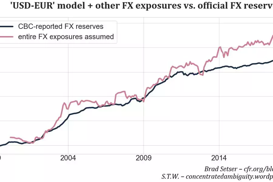
Corroborating the abstracted indications obtained during the setup phase, Fig. 15 shows just how suitable this model of relying on the CBC’s PnL to draw inferences about its FX exposure is. The created time series of the CBC’s FX exposures is highly correlated in level terms with the CBC’s officially released FX reserves. Slight deviations during 2003, 2007 and 2012 exist, are however short-lived and tend to be corrected in the ensuing months.

This pattern breaks starting in 2014, after which the indicated FX exposures of the CBC continuously exceed the level implied by its FX reserves. This is exactly what would be expected if a central bank is indeed intervening in FX markets to weaken its currency via FX derivatives—in this case by swapping FX obtained from outright interventions with a local counterparty. The difference between the calculated FX exposure and reported FX reserves in turn represents the central bank’s estimated FX derivative exposure.

In Taiwan’s case, the results implied by USD and EUR currency factors alone indicate excess FX exposures created via FX swaps of ∼USD 65bn as of mid-2018. Already a meaningful sum, this amount is set to grow further when incorporating the remaining currencies which were so far set aside in this section’s model.

F. AUD, JPY & Co—Incorporating Remaining FX Exposures

In order to comprehend the entirety of a central bank’s intervention in FX markets, all its FX exposures have to be aggregated. As shown in the left half of Fig. 16, this requires the summation of (1) the FX exposures in each currency it holds as on-balance sheet FX reserves, as well as (2) any exposures arising from transactions in FX derivatives. Given that FX reserves are predominantly denominated in USD or EUR, these currencies naturally form the largest portion of FX exposures created by accumulating on-balance sheet FX reserves. Despite this primacy, a group of other currencies (including AUD, JPY, GBP, CAD, CHF, AUD, CNY) have in the past decade almost doubled their share in the currency composition of global FX reserves reported in the IMF’s COFER survey, now accounting for ∼18%. No currency denominations are available for interventions via FX derivatives, yet anecdotal evidence strongly suggests these mostly are conducted against USD. In Taiwan’s case, this is practically guaranteed, as the CBC provides FX hedges to lifers, which, as shown in the second blog this series, conduct their foreign business almost exclusively in USD—and thus require USD FX hedges.

Optimally, all individual FX exposures would be measured in a single step, which would be synonymous to the inclusion of all currencies in the regression exercise in the prior blog (part four). Unfortunately, this is practically infeasible for a simple reason: While the USD and EUR exposures of the CBC are large enough to trace effects on its PnL, the remaining currencies account for a much smaller share of FX exposures and are thus not reliably picked up by the models in the previous section. Further, the inclusion of many correlated currencies may, at times, raise serious issues of multicollinearity.

For these reasons, it was decided to only include USD and EUR variables in the main model and postpone the inclusion of other currency exposures until now. As most central banks, the CBC does not provide a breakdown of the currency composition of its FX reserves. In its monthly FX reserve statements, it nonetheless frequently references FX market moves in JPY, GBP and other currencies affecting the valuation of its FX reserves when expressed in USD^[30] and states its FX reserve “composition is similar to those of other major central banks around the world.”^[31]

Consequently, it will be assumed the CBC’s allocation of currencies other than USD and EUR in its on-balance sheet FX reserves follows the global average of all central banks, values for which are obtained from the quarterly IMF COFER survey.

The incorporation of currencies other than the euro and the dollar is slightly more difficult than a cursory look might suggest. This is due to possible correlation effects between the referenced currencies crossed against TWD, which may lead to portions of other currencies indirectly already being accounted for by the ’USD-EUR’ model in the prior section. The right-half of Fig. 16 serves to indicate such dynamics: The ’USD-EUR’ model certainly covers FX exposures resulting from FX reserves kept in either of the two currencies, plus the FX derivative exposure taken via FX swaps, which are USD-denominated. In addition, and depending on how correlated a given currency is with the USD and EUR variables during a specific time frame, varying portions of the smaller currencies’ shares may also already be accounted for by the ’USD-EUR’ model.

The dynamics may be best illustrated by an example. From mid-2012 through mid-2014, strong demand to convert EUR into CHF, as a consequence of the Euro crisis, led the Swiss National Bank to ’floor’ the EURCHF exchange rate at 1.20 CHF per Euro. As a result, the FX pair spent these two years in a very narrow channel just above the 1.2 floor, with minimal volatility. A byproduct of this temporary quasi-peg and the ensuing tranquility in this specific FX cross is that EUR and CHF will exhibit an extremely high correlation, when measured against a common third currency, e.g. EUR/TWD and CHF/TWD show very high co-movements.

The problem of the correlation is that while the ‘USDEUR’ model explicitly accounts for FX exposures in these currencies, the indistinguishable returns of EUR/TWD and CHF/TWD will make it also measure exposures to the latter cross, and hence allocations of FX reserves denominated in CHF. For this reason, simply adding COFER implied CHF FX exposures to the ’USD-EUR’ model could lead to potential double counting and overstatements of overall FX exposures. Instead, the correlation effects of each currency with USD and EUR variables will have to be considered as well. Equations (6) and (7) show the procedure formulaically,

where N is the number of currencies FX reserves are held in apart from USD and EUR. A single currency’s contribution is then calculated as

Per Equation (6), the CBC’s overall FX exposures at a specific point in time are the already known coefficients for USD and EUR, supplemented by the FX exposures from other currencies FX reserves are held in. Equation (7) details the calculation of the contribution of a single currency i in this basket at a specific point in time. The starting point is the currency’s share in the IMF COFER survey. This value is multiplied by currency i’s uncorrelated movement with the USD & EUR variables, calculated as 1 − r² of a bivariate regression of currency i’s returns during a specific 22 month time frame on USD and EUR returns^[32]. If a currency is highly correlated with USD or EUR, 1 − r² will be small, thus lowering the (additional) contribution of this currency. In fact, it is not really lowering the currency’s contribution, as much as avoiding double counting of exposures which, due to high correlations, have already been accounted for by the ’USD-EUR’ model. Lastly, the percentage share will have to be scaled by the current size of the CBC’s FX reserves to attain a nominal USD value.

As an example, at the end of 2017, GBP made up ∼5% of FX reserves in the IMF COFER survey. During the 22 month time frame which is divided into equal parts by December 2017, 17% of the variation in GBP/TWD can be explained by movements in USD/TWD and EUR/TWD. Subtracting this figure from 100% and multiplying by the COFER share yields 0.05 × 0.83 = 0.0415, which is the percentage of official FX reserves to be added on top of the ’USD-EUR’ model to account for not yet included GBP exposures. Multiplying this share by the size of the CBC’s reported FX reserves of USD 451bn in December 2017 results in a nominal value of USD 18.71bn.

Repeating this process systematically for all currencies included in the IMF COFER survey and for every single month starting in 2001 yields the following results:

The top panel in Fig. 17 shows the allocation to currencies^[33] other than USD and EUR in the IMF COFER survey; the lower panel shows the evolution of explained variance of returns by the relevant currencies crossed against TWD by USD/TWD and EUR/TWD returns. Also shown is the average of these time series, which will be applied to the ’other’ currencies category, which is not described in more detail in the IMF COFER survey.

The upper panel in Fig. 18 shows the percentage share of FX reserves per currency to be added on top of the ’USD-EUR’ model, calculated as the upper panel in Fig. 17 × (1 - the lower panel). The bottom panel in Fig. 18 translates these into nominal USD values by multiplying by the respective size of Taiwan’s reported FX reserves at each point in time.

In a final step, these additional FX exposures to other currencies will be added on top of the ’USD-EUR’ model in order to create the final result presented in Fig. 19.

As in the ’USD-EUR’ model before, the measured overall FX exposures of the CBC are tightly correlated with its official FX reserves up through 2010—the time period before lifers became active buyers in foreign markets & acquirers of large amounts of FX hedges. Thereafter, the time series clearly diverge. From 2011 through mid-2018, the CBC’s FX reserves increased by USD 70bn only; the measured FX exposures in contrast by USD 160bn, a difference of USD 90bn.

As discussed, deviations in these time series can be attributed to FX exposures assumed via FX derivatives. With the background of the prior blogs, including the obvious demand for FX hedges by lifers and the lack of (sufficiently large) counterparties to their position by private sector actors, it seems self-evident that the continued rise in the CBC’s FX exposures is explained by it taking the other side of lifers’ FX hedges via currency interventions in the FX swap market.

Based on the central tendency produced by the latest estimate for mid-2018, the CBC’s FX swap book—and ipso facto its hitherto undisclosed FX interventions—amounts to ∼USD 130bn.

G. Testing the CBC’s FX Swap Book for Significance

The modeling results displayed in Fig. 19 show the central tendency produced when estimating the CBC’s overall FX exposure. For every month, the same model setup described in prior sections is run using 22 months of data to calculate the USD and EUR coefficients, to which exposures in other currencies are later added, after their co-variation with the directly included currencies is stripped off.

As with any statistical model, knowledge of the central tendency is a required first step, it should however be immediately followed by testing results for statistical significance. If for instance the model’s errors are large, it could be conceivable that the gap between the CBC’s FX exposures and its published FX reserves is attributable to statistical errors rather than a genuine divergence in reality.

There are several ways to show that the model results—and in consequence the divergence between the two time series—are of high quality and unlikely due to pure chance.

First, the r² values reported by the ’USD-EUR’ model average north of 0.9, meaning that the true variation in the CBC’s local currency PnL can be almost entirely explained by these two factors alone. Since standard errors of single coefficients in a regression are, among other things, determined by the overall fit of the entire model, it stands to reason that errors in the USD and EUR coefficients will not be overly large.

Second, the results in Fig. 19 are not the outcome of a single application of the model, but rather of many rolling window calculations. If the modeled FX exposures then exceed the FX reserve numbers permanently—particularly in windows with little or no overlap in data inputs—it is probable that the mid-point estimates are of high quality and not due to random errors. If the latter were the case, wild fluctuations (both above and below the FX reserve values) in the FX exposure time series would be expected. In reality, the modeled FX exposures exceed the reported FX reserves in more than 94% of all considered months. Further, the resulting time series is fairly steady, alleviating concerns that it is randomness creating the divergence.

Lastly and most formally, estimates for the errors of individual components of the model can be combined to create confidence intervals for the CBC’s total ’true’ FX exposure. If the CBC’s reported FX reserves lie outside of a specific confidence interval, the CBC’s FX swap interventions can be classified as statistically significant at the specified confidence level.

Standard errors for USD and EUR are readily available from the regression setup (see in Fig. 14 previously) and only have to be converted into USD and shifted back 11 months in time^[34]. Given no indications to the contrary, the error structure will be assumed to be uncorrelated, so the combined standard error of these is simply the square root of the sum of their individual variances.

The standard errors for the other currencies are more difficult to assess. Since the CBC does not release its currency compositions directly, the starting point for these are the point values taken from the IMF COFER survey. How well they match the true CBC allocations is hard to say, so as an alternative, the spread of individual countries around the aggregate COFER value will be taken as a guide for the variability. Most countries of course do not release such values, but strong evidence exists nonetheless^[35], indicating that the spread around the COFER implied allocations is small. Erring on the side of caution, it will be assumed that the standard deviation of the CBC’s allocation to currencies other than USD and EUR is 20% of the actual allocation. For the latest available data, this implies a mid-point estimate of 18% and a standard deviation of 3.5%, which translates into a 95% interval of between 10.5% and 25%. On the downside, this seems more than conservative given the CBC’s frequent mentions of the influence other currencies have on the valuation of its FX reserves when expressed in USD.

Fig. 20 shows the results when the estimated errors in the other currencies (again assuming uncorrelated errors) are added to the directly obtained standard errors from the ’USDEUR’ model. The three gray-colored channels surrounding the central tendency represent confidence intervals at the 90%, 95% and 99% levels respectively. The lower panel indicates instances in which the CBC’s published FX reserves lie outside a specific confidence interval, progressively indicating increasing levels of statistical significance.

Since late 2014, excess FX exposures by the CBC acquired via its FX swap book are at a minimum significant at the 10% level; since late 2015 significance increased further, coming in at the 1% level most of the time, including the last year of available data, during which this is consistently the case.

Joining these numerical results with the CBC’s self-reported qualitative acknowledgment of its activities in FX derivative markets, the case for hitherto non-public interventions in FX markets via its FX swap book seems overwhelming. This is particularly the case in the broader context—Taiwan’s life insurance industry has a large disclosed FX hedging need, and, as the previous blogs have illustrated, neither Taiwan’s banks nor non-residents appear to be potential counterparties for the full hedging need. The scale of this undisclosed intervention appears quite large—at least $130 billion, and perhaps as large as $200 billion. Intervention on this scale over the past six years helps explain the remarkable stability of the Taiwan dollar. Taiwan’s undisclosed intervention, is also large enough to materially change, among other things, the U.S. Treasury’s assessment of Taiwan in its semi-annual foreign exchange report.

 

 

* The Council on Foreign Relations takes no institutional positions on policy issues and has no affiliation with the U.S. government. All views expressed on its website are the sole responsibility of the author or authors.The Council on Foreign Relations takes no institutional positions on policy issues and has no affiliation with the U.S. government. All views expressed on its website are the sole responsibility of the author or authors.
** Contact at [email protected]

[1] Which can be found here.
[2] Since FX swaps can be decomposed into its individual components, it is of course possible, in theory, to transform a package of these into having outright FX exposure, by adding further spot or forward transactions.
[3]Given that lifers rely on FX swaps to hedge the largest part of their FX exposures, the most probable reason for the CBC to intervene via swaps is to ease the burden on the banking system, which can simple match up the demand for FX swaps by lifers with the supply of the CBC. If the CBC only wrote forwards to banks, they would need to decompose the swap into its components, requiring balance sheet space and thus (slightly) increasing the cost for lifers. Specifically, banks would need to expand their balance sheets by borrowing additional TWD, exchange these for USD. This would create balance regarding the CBC leg. They would then swap-lend USD to lifers, in return for TWD. At trade conclusion, these are reversed, the bank again has an on-balance sheet mismatch, leaving it long USD, which is countered by its long TWD position obtained by the forward transaction with the CBC.
[4] In this case, it is assumed banks simply keep excess TWD liquidity on deposit with the CBC. Other modes of sterilization like CBC bills, repos or government bond issuance are equally conceivable.
[5] This explanatory sequence seeks to understand the logical chain of transactions required to provide lifers with FX swaps. It is possible the sequentiality might (falsely) suggest longer time distances between these steps. This is not the case. In practice, once an insurer enters into the first transaction with the bank, the subsequent transactions are all entered simultaneously (or immediately thereafter) in order to achieve same day settlement, leaving the intermediating bank FX neutral at all times.
[6] This upward revision would then accurately portray the size of the CBC’s FX exposures, but the jump in reserves the observer sees when the swap is unwound does not reflect the timing of the CBC’s intervention accurately. The increase in FX exposures took place in step II, which was however obscured, since in step III immediately thereafter, the CBC’s balance sheet shrank due to the swap transaction.
[7] Moreno, R (2011):’Foreign exchange market intervention in EMEs: implications for central banks’, BIS Papers, vol 57, pp 65–86.
[8] Basis risk is the non-negligible edge case.
[9] In the simplest of all cases, assume the value of a fund share always increases 0.5% for every 1% move up in stock A, and vice versa. It is clear then that the manager’s exposure to stock A is 0.5×100=50% of AuM.
[10] As with most regressions, it is not only coefficients which are returned, but also confidence intervals for these, as well as global goodness-of-fit characteristics for the entire exercise.
[11] And in all likelihood the denomination of FX derivative exposures.
[12] Or if known, more suitable regional indices reflecting the C.B.’s allocation.
[13] This would require knowledge about the currency composition and asset composition of the central bank’s FX reserves. Since these are however only uncovered via this exercise, it is easiest to treat the FI arbitrage PnL as residual of the regression.
[14] Which would be equivalent to the CBC’s net worth, if viewed from a private sector angle.
[15] As also evidenced by the lack of volatility in the equity time series. The same lack of volatility is also found in the value of FX reserves on the asset side of its balance sheet.
[16] Because the CBC’s balance sheet more than quadrupled during this timeframe, directly calculating the correlation of the upper panel is inadvisable. A much better view is attained by calculating rolling window correlations on the changes in the variables, thus capturing the time-varying nature of the CBC’s FX reserve holdings. As a result of this growth, in the late 2000s, even small fluctuations in FX markets already had a marked impact on the CBC’s equity.
[17] This would clearly have been felt by market participants at the time, plus the central bank would clearly have had an incentive to provide the public clarity around such a large shift in policy.
[18] Available here.
[19] It is not exactly equivalent, since the CBC’s equity statement is not flat but exhibits the previously described pattern.
[20] The risk of an overly complex model would lie in spurious factors distorting the effects assigned to truly significant variables. Since this entire exercise is predicated on measuring a central bank’s FX exposure by the size of the coefficients of variables in a regression framework, inclusion of variables should be carefully weighed.
[21] That is, each month, a regression is run using the past 22 months of data, creating a single r² value for this particular segment. This exercise is repeated for every consecutive month, sliding the rolling window one month forward. Averaging all attained r² values provides a good estimation of a factor's importance in explaining the CBC’s PnL.
[22] By correctly signed, it is meant that an increase in the relevant currency vs. TWD leads to a positive PnL for the CB—as would be dictated by the CBC being long foreign currencies. For equity and duration factors, correctly signed implies a long exposure. This sign restriction can guard against spurious correlation.
[23] The lack of observable long exposure to U.S. bonds is notable (this also holds when adding the duration factor to the optimal USD & EUR setup) and counter to the duration exposure of other central banks. It could be due to the CBC not marking its FI holdings to market. The more likely reason however is that the CBC relies on very short-dated assets, as confirmed on its website: “The bulk of these foreign exchange reserves are deposited in overseas banks[...].”
[24] It is important to keep in mind that because the USD variable is highly significant, a currency (say X) with low volatility (or at the extreme, a peg) when crossed against USD would score highly in this exercise simply because USD/TWD would be highly correlated with X/TWD. None of the currencies is highly correlated with USD, but it might be a factor for CAD.
[25] CHF comes close, but its quasi peg to EUR is the much more likely reason than outsized exposures to CHF.
[26] This materializes by the regression maximizing the explanatory power by utilizing the entire cross section of variables it is provided. As a result, it tends to create ’long-short’ positions in multiple variables, which are highly unstable. For instance, if in one specific 22 month time frame, the AUD-CHF exchange rate has some coincidental predictive power for the CBC’s PnL, the regression would assign very large positive values to AUD and the opposite to CHF. Given that these are most likely spurious, they would be ’unwound’ in a later period. Such misattributions can also affect the coefficients of truly significant variables, thus it is best to just limit model complexity and stay with the USD and EUR variables. Regularization methods might be of help in a single static regression; in the rolling window context, however, their application is less helpful.
[27] For instance assume a 12m window is selected. If however FX markets are unchanged during, say, 5m of these, the effective window is rather 7m. Including the two explanatory variables and the intercept, that is only 4 degrees of freedom, potentially opening the door to too high month-over-month volatility in the coefficients.
[28] This would occur for instance if the FX effect of each currency were to be split into three components: the current 1m rate of change, as well as two lagged versions of it, reflecting changes one or two months prior.
[29] To be precise, the regression not only captures the FX exposures arising from USD or EUR allocations, but also any other currency’s unorthogonal variation with either. This topic will be explored shortly, in the context of accounting for the currencies not directly included in the regression discussed here.
[30] See for instance here.
[31] Quoted from here.
[32] This process can also be approached visually, from a linear algebra perspective. For any particular 22 month period, the USD and EUR variables form a plane in a 22 dimensional space. By solving the linear equation, this plane is mapped (as best as possible) to a line representing the CBC’s PnL. If a third currency is highly correlated with USD, EUR or a combination thereof, the currency’s return vector lies largely in the plane spanned by USD and EUR returns—consequently it does not add much new information to the system’s column space and its correlated exposures would have been picked up by the USD and EUR variables anyway. Instead of calculating 1− r² for each currency, it would also be possible to calculate the third currency’s length orthogonal to the ’USD-EUR’ plane and divide it by its entire length.
[33] In recent years, allocations to CNY-denominated assets have risen and are currently stated at 1.95% of COFER-reported FX reserve assets. Since Russia accounts for a large portion of such holdings and Taiwan is for geopolitical reason unlikely to hold Mainland Chinese assets, allocations to CNY assets in the IMF survey will be replaced by scaling up the other here included currencies proportionally.
[34] In order to align with coefficients, which were shifted back in an earlier section already.
[35] Before 2015, the IMF released two additional datasets on currency allocations of FX reserve managers in Advanced and Emerging economies respectively. The allocation to other currencies in both were very similar throughout time. In addition, since 2015 three of the biggest FX reserve mangers (China, Saudi Arabia and Russia) have joined the IMF panel. The inclusion of none of these shifted the overall mix in the world survey materially, implying that their allocations are about in line with countries already included in the survey.
[36] The standard error for the other currencies is, of course, calculated by applying the 20% variation to the orthogonal variation, unexplained by the ’USD-EUR’ model. The standard errors for correlated exposures are already accounted for in the uncertainty calculated for the USD and EUR coefficients.